Antenna main technical data and their meanings

1.Gain

Gain is a crucial parameter that quantifies the power concentration of an antenna. It represents the ratio of the power density produced by the actual antenna to that of an ideal radiating element at the same point in space, assuming equal input power. The antenna’s gain is directly influenced by its pattern – a narrower main lobe results in smaller side lobes and higher gain.

The physical meaning of gain can be illustrated as follows: To transmit a signal of a specific size over a certain distance, an ideal non-directional point source requires 100W input power. However, if a directional antenna with a gain of G = 13 dB = 20 is used as the transmitting antenna, the input power needed is only 100 / 20 = 5W. In essence, the antenna’s gain indicates the multiple times of input power amplification in its maximum radiation direction compared to an ideal point source with no directivity.

The gain of the half-wave symmetric oscillator is 2.15 dBi.

The arrangement consists of four half-wave symmetry oscillators positioned along a vertical line to form a vertical quaternion array, with an approximate gain of G=8.15dBi (the unit dBi indicates the comparison to an ideal point source with uniform radiation in all directions).

When using a half-wave symmetry oscillator as the reference, its gain is measured in dBd. The gain of a half-wave symmetry oscillator is G=0dBd (since it is self-sufficient with a ratio of 1, resulting in a logarithm of zero). The vertical quaternion array achieves a gain of approximately G=8.15–2.15=6dBd.

2. Beam width

The radiation pattern of an antenna typically exhibits multiple lobes, with the highest radiance known as the main lobe and the others referred to as side lobes. In Figure 1.3.4a, the angle between the two points where the radiation intensity decreases by 3 dB (half the power density) on either side of the main lobe’s maximum radiation direction is defined as the lobe width (also called beam width, main lobe width, or half-power angle). A narrower lobe width indicates better directivity, increased action distance, and stronger anti-interference capability.

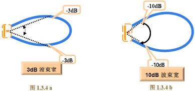
Additionally, there is another parameter known as the 10 dB lobe width. As the name suggests, it represents the angle between two points in the radiation pattern where the radiation intensity decreases by 10 dB (equivalent to reducing the power density to one-tenth), as illustrated in Figure 1.3.4b.

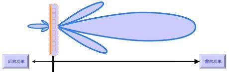
3.Front-To-Back Ratio

The ratio of the maximum value of the radiation intensity in the forward lobe to that in the backward lobe is known as the front-to-back ratio (F/B), expressed as F/B = 10 * log10 {(forward power density) / (backward power density)}. A higher front-to-back ratio indicates reduced backward radiation (or reception) of the antenna.

Calculating the front-to-back ratio (F/B) is straightforward, and when required for an antenna, typical values range between (18 ~ 30) dB. In special cases, the front-to-back ratio may need to reach (35 ~ 40) dB.

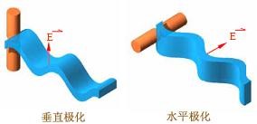
4．Polarization of the antenna

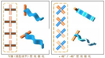
The antenna emits electromagnetic waves into the surrounding space, which consist of an electric field and a magnetic field. The polarization direction of the antenna is defined by the direction of the electric field. Most commonly used antennas are unipolar. The illustration below depicts two fundamental single-polarization cases: vertical polarization – the most common, and horizontal polarization – also commonly used.

4.1 Dual polarized antenna

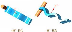
The illustration below presents two additional cases of single polarization: +45° polarization and -45° polarization, which are reserved for special applications. Consequently, four types of single polarization antennas are available, as depicted in the figure below. When two polarized antennas of vertical and horizontal polarization are combined, or when two polarization antennas of +45° and -45° polarization are combined, they form a new type of antenna known as a double-polarized antenna.

In the illustration below, two single-polarized antennas are mounted together, creating a dual-polarized antenna. It’s important to note that a dual-polarized antenna is equipped with two connectors. This type of antenna emits (or receives) two waves that are spatially orthogonal (i.e., perpendicular) to each other, typically one in the vertical and the other in the horizontal direction.

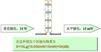
4.2 Polarization isolation

In practice, achieving perfect polarization isolation is challenging. When a signal is fed into a polarized antenna, a small portion of it will inevitably leak into another polarized antenna. For instance, in the dual-polarized antenna depicted below, if the input power for the vertically polarized antenna is 10W, the measured output power at the horizontally polarized antenna’s output will be 10mW.

5 Antenna input impedance-Zin

Definition: The input impedance of an antenna refers to the ratio of the signal voltage at the antenna’s input to the signal current. It comprises a resistance component (Rin) and a reactance component (Xin), represented as Zin = Rin + jXin. The presence of the reactive component leads to a reduction in signal power extraction from the feeder. Hence, efforts are made to minimize the reactance component, aiming for a purely resistive input impedance for the antenna. However, even a well-designed and tuned antenna typically exhibits a small reactance component in its input impedance.

The input impedance is influenced by the antenna’s structure, size, and operating wavelength. For instance, the half-wave symmetric oscillator is a fundamental antenna with an input impedance of Zin = 73.1 + j42.5 ohms (Europe). By slightly shortening its length (3~5%), the reactance component can be eliminated, resulting in a pure resistive input impedance of Zin = 73.1 ohms (Europe) or the nominal 75 ohms. However, this purely resistive impedance is only applicable to a specific frequency.

On the other hand, the half-wave folded oscillator has four times the input impedance of the half-wave symmetric oscillator, i.e., Zin = 280 ohms (nominal 300 ohms).

It’s worth noting that any antenna can be adjusted through impedance tuning. Ideally, in the required operating frequency range, the input impedance should have a small imaginary part and be quite close to 50 ohms in real part, resulting in Zin = Rin = 50 ohms. This impedance matching with the feeder is vital for optimal antenna performance.

6 Antenna operating frequency range (bandwidth)

In both transmitting and receiving antennas, they function within a specific frequency range, known as the antenna’s bandwidth. There are two different definitions for the bandwidth:

The working frequency bandwidth of the antenna under the condition of a standing wave ratio (SWR) ≤ 1.5.
The bandwidth over which the antenna gain drops within 3 decibels.

In mobile communication systems, the first definition is commonly used. Thus, the antenna’s bandwidth refers to the frequency range in which the antenna operates with a standing wave ratio (SWR) not exceeding 1.5.

It is important to note that antenna performance can vary at different frequency points within the operating frequency bandwidth. However, such performance variations are generally acceptable as long as they do not lead to significant degradation in performance.

7. Several basic concepts of transmission lines

The cable that connects the antenna to the transmitter output (or receiver input) is known as a transmission line or feeder. Its primary function is to efficiently transmit signal energy. Therefore, it should minimize signal loss while transmitting the signal power from the transmitter to the input of the transmitting antenna or from the antenna to the receiver input. At the input end, the transmission line must be shielded to avoid picking up or generating unwanted interference signals.

By the way, when the physical length of the transmission line equals or exceeds the wavelength of the transmitted signal, it is also referred to as a long line.

7.1 Type of transmission line

There are generally two types of ultra-short-band transmission lines: parallel two-line transmission lines and coaxial cable transmission lines. In the microwave band, transmission lines include coaxial cable transmission lines, waveguides, and microstrips.

A parallel two-wire transmission line consists of two parallel conductors and is symmetrical or balanced. However, this type of feeder has significant loss and is unsuitable for use in the UHF band.

On the other hand, a coaxial cable transmission line comprises a core wire and a shielded copper mesh. As the copper mesh is grounded, the two conductors become asymmetric to the ground, making it an asymmetric or unbalanced transmission line. Coaxial cables offer a wide operating frequency range, low loss, and provide some shielding against electrostatic coupling.

However, they may be susceptible to interference from magnetic fields. During usage, it is essential to avoid parallel installation with lines carrying strong currents and maintain distance from low-frequency signal lines.

7.2 Characteristic impedance of the transmission line

The characteristic impedance of a transmission line, denoted by Z0, is the ratio of voltage to current along an infinitely long line.

Typically, Z0 has two common values: Z0 = 50 ohms and Z0 = 75 ohms.

The characteristic impedance of the feeder depends solely on the conductor diameters D and d, as well as the dielectric constant εr of the material between the conductors. It remains constant and is not affected by the feeder’s length, operating frequency, or the load impedance at the feeder’s terminal.

7.3 Feeder attenuation coefficient

In a feeder, the signal transmission results in two types of losses: resistive loss in the conductor and dielectric loss in the insulating material. As the feeder length and operating frequency increase, these losses also increase. Hence, it is advisable to minimize the length of the feeder.

The loss per unit length is quantified by the attenuation coefficient (β), typically expressed in dB/m (decibels per meter), or in technical specifications, as dB/100m (decibels per 100 meters) for cables. For instance, a NOKIA 7/8 inch low-consumption cable exhibits an attenuation factor of β = 4.1 dB/100m at 900 MHz, which can also be expressed as β = 3 dB/73m. This means that for every 73 meters of this cable, the signal power at 900 MHz reduces to less than half.

On the other hand, ordinary non-low-cost cables, like SYV-9-50-1, have an attenuation coefficient of β = 20.1 dB/100m at 900 MHz, or β = 3 dB/15m. In this case, for every 15 meters of this cable at 900 MHz, the signal power becomes less than half of the power of the original signal.

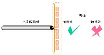
7.4 Matching concept

What is a match? Simply put, when the load impedance ZL connected to the feeder terminal is equal to the feeder characteristic impedance Z0, it is called the feeder terminal is matched. When matching, there are only incident waves on the feeder that are transmitted to the terminal load, and there is no reflected wave generated by the terminal load. Therefore, when the antenna is used as the terminal load, the matching can ensure that the antenna obtains all signal power.

As shown in the figure below, when the antenna impedance is 50 ohms, it matches the 50 ohm cable, and when the antenna impedance is 80 ohms, it does not match the 50 ohm cable.

If the antenna oscillator has a relatively large diameter, its input impedance remains relatively stable across frequencies, making it easier to achieve a good match with the feeder. Consequently, the antenna can operate over a broader frequency range. Conversely, antennas with smaller diameters may have a narrower operating frequency range.

In practical applications, the input impedance of the antenna can also be influenced by surrounding objects or the environment. To ensure a proper match between the feeder and the antenna, adjustments to the local structure of the antenna or the installation of a matching device may be necessary during antenna measurements and installations. These measures help optimize the antenna’s performance and ensure efficient signal transfer.

8. Voltage standing wave ratio（VSWR）

In the case of a mismatch, both incident and reflected waves are present on the feeder. When the phase of the incident wave and the reflected wave are the same, their voltage amplitudes add up, resulting in an antinode with the maximum voltage amplitude (Vmax). Conversely, when the incident wave and the reflected wave are in opposite phases, their voltage amplitudes subtract, forming a node with the minimum voltage amplitude (Vmin). Amplitude values at other points lie between the antinode and the node. This combined wave pattern is known as a standing wave.

A smaller reflection coefficient (R) and a standing wave ratio (VSWR) closer to 1 indicate better matching between the terminal load impedance (ZL) and the characteristic impedance (Z0) of the feeder. As the terminal load impedance approaches the characteristic impedance, the mismatch decreases, resulting in reduced reflection and improved matching.